audioflux.linear_spectrogram

audioflux.linear_spectrogram(X, num=None, radix2_exp=12, samplate=32000, slide_length=None, low_fre=0.0, window_type=WindowType.HANN, style_type=SpectralFilterBankStyleType.SLANEY, data_type=SpectralDataType.POWER, is_reassign=False)

Short-time Fourier transform (Linear/STFT)

It is a Fourier-related transform used to determine the sinusoidal frequency and phase content of local sections of a signal as it changes over time.

Note

We recommend using the BFT class, you can use it more flexibly and efficiently.

Parameters

X: np.ndarray [shape=(…, n)]

audio time series.

num: int or None

Number of frequency bins to generate, starting at low_fre.

If num is None, then num = fft_length / 2 + 1. When radix2_exp=12, fft_length=4096, samplate=32000, low_fre=0, then num=2049, and frequency range is 0-16000.

The size of each band is samplate / fft_length.

radix2_exp: int

fft_length=2**radix2_exp.

samplate: int

Sampling rate of the incoming audio.

slide_length: int or None

Window sliding length.

If slide_length is None, then slide_length = fft_length / 4

low_fre: float

Lowest frequency.

window_type: WindowType

Window type for each frame.

See: type.WindowType

style_type: SpectralFilterBankStyleType

Spectral filter bank style type. It determines the bank type of window.

see: type.SpectralFilterBankStyleType

data_type: SpectralDataType

Spectrogram data type.

It cat be set to mag or power. If you needs db type, you can set power type and then call the power_to_db method.

See: type.SpectralDataType

is_reassign: bool

Whether to use reassign.

Returns

spectrogram: np.ndarray [shape=(…, fre, time)]

The matrix of Linear(STFT)

fre_band_arr: np:ndarray [shape=(fre,)]

The array of frequency bands

See also

mel_spectrogram

bark_spectrogram

erb_spectrogram

BFT

NSGT

CWT

PWT

Examples

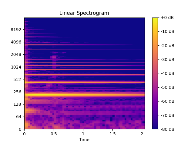
Read 220Hz audio data

>>> import audioflux as af
>>> audio_path = af.utils.sample_path('220')
>>> audio_arr, sr = af.read(audio_path)

Extract spectrogram of dB

>>> low_fre = 0
>>> spec_arr, fre_band_arr = af.linear_spectrogram(audio_arr, samplate=sr, low_fre=low_fre)
>>> spec_dB_arr = af.utils.power_to_db(spec_arr)

Show spectrogram plot

>>> import matplotlib.pyplot as plt
>>> from audioflux.display import fill_spec
>>> import numpy as np
>>>
>>> # calculate x/y-coords
>>> audio_len = audio_arr.shape[-1]
>>> x_coords = np.linspace(0, audio_len/sr, spec_arr.shape[-1] + 1)
>>> y_coords = np.insert(fre_band_arr, 0, low_fre)
>>>
>>> fig, ax = plt.subplots()
>>> img = fill_spec(spec_dB_arr, axes=ax,
>>>                 x_coords=x_coords,
>>>                 y_coords=y_coords,
>>>                 x_axis='time', y_axis='log',
>>>                 title='Linear Spectrogram')
>>> fig.colorbar(img, ax=ax, format="%+2.0f dB")