Spectral
- class audioflux.Spectral(num, fre_band_arr)
Spectrum feature, supports all spectrum types.
- Parameters
- num: int
Number of frequency bins to generate. It must be the same as the num parameter of the transformation (same as the spectrogram matrix).
- fre_band_arr: np.ndarray [shape=(n_fre,)]
The array of frequency bands. Obtained by calling the get_fre_band_arr() method of the transformation.
Methods
band_width(m_data_arr[, p])Compute the spectral band_width feature.
broadband(m_data_arr[, threshold])Compute the spectral broadband feature.
cd(m_data_arr, m_phase_arr)Compute the spectral cd feature.
centroid(m_data_arr)Compute the spectral centroid feature.
crest(m_data_arr)Compute the spectral crest feature.
decrease(m_data_arr)Compute the spectral decrease feature.
eef(m_data_arr[, is_norm])Compute the spectral eef feature.
eer(m_data_arr[, is_norm, gamma])Compute the spectral eer feature.
energy(m_data_arr[, is_log, gamma])Compute the spectral energy feature.
entropy(m_data_arr[, is_norm])Compute the spectral entropy feature.
flatness(m_data_arr)Compute the spectral flatness feature.
flux(m_data_arr[, step, p, is_positive, ...])Compute the spectral flux feature.
hfc(m_data_arr)Compute the spectral hfc feature.
kurtosis(m_data_arr)Compute the spectral kurtosis feature.
max(m_data_arr)Compute the spectral max feature.
mean(m_data_arr)Compute the spectral mean feature.
mkl(m_data_arr[, tp])Compute the spectral mkl feature.
novelty(m_data_arr[, step, threshold, ...])Compute the spectral novelty feature.
nwpd(m_data_arr, m_phase_arr)Compute the spectral nwpd feature.
pd(m_data_arr, m_phase_arr)Compute the spectral pd feature.
rcd(m_data_arr, m_phase_arr)Compute the spectral rcd feature.
rms(m_data_arr)Compute the spectral rms feature.
rolloff(m_data_arr[, threshold])Compute the spectral rolloff feature.
sd(m_data_arr[, step, is_positive])Compute the spectral sd feature.
set_edge(start, end)Set edge
set_edge_arr(index_arr)Set edge array
set_time_length(time_length)Set time length
sf(m_data_arr[, step, is_positive])Compute the spectral sf feature.
skewness(m_data_arr)Compute the spectral skewness feature.
slope(m_data_arr)Compute the spectral slope feature.
spread(m_data_arr)Compute the spectral spread feature.
var(m_data_arr)Compute the spectral var feature.
wpd(m_data_arr, m_phase_arr)Compute the spectral wpd feature.
- set_time_length(time_length)
Set time length
- Parameters
- time_length: int
- set_edge(start, end)
Set edge
- Parameters
- start: int
0 ~ end
- end: int
start ~ num-1
- set_edge_arr(index_arr)
Set edge array
- Parameters
- index_arr: np.ndarray [shape=(n,), dtype=np.int32]
fre index array
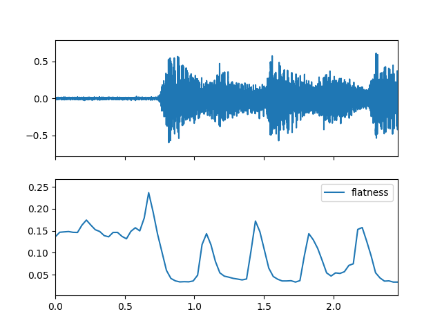
- flatness(m_data_arr)
Compute the spectral flatness feature.
\(\qquad flatness=\frac{\left ( \prod_{k=b_1}^{b_2} s_k \right)^{ \frac{1}{b_2-b_1} } } {\frac{1}{b_2-b_1} \sum_{ k=b_1 }^{b_2} s_k}\)
\(b_1\) and \(b_2\): the frequency band bin boundaries
\(s_k\): the spectrum value, which can be magnitude spectrum or power spectrum
- Parameters
- m_data_arr: np.ndarray [shape=(…, fre, time)]
Spectrogram data.
- Returns
- flatness: np.ndarray [shape=(…, time)]
flatness frequency for each time
Examples
Read chord audio data
>>> import audioflux as af
>>> audio_path = af.utils.sample_path('guitar_chord1')
>>> audio_arr, sr = af.read(audio_path)
Create BFT-Linear object and extract spectrogram
>>> from audioflux.type import SpectralFilterBankScaleType, SpectralDataType
>>> import numpy as np
>>> bft_obj = af.BFT(num=2049, samplate=sr, radix2_exp=12, slide_length=1024,
>>>                data_type=SpectralDataType.MAG,
>>>                scale_type=SpectralFilterBankScaleType.LINEAR)
>>> spec_arr = bft_obj.bft(audio_arr)
>>> spec_arr = np.abs(spec_arr)
Create Spectral object and extract flatness feature
>>> spectral_obj = af.Spectral(num=bft_obj.num,
>>>                            fre_band_arr=bft_obj.get_fre_band_arr())
>>> n_time = spec_arr.shape[-1]  # Or use bft_obj.cal_time_length(audio_arr.shape[-1])
>>> spectral_obj.set_time_length(n_time)
>>> flatness_arr = spectral_obj.flatness(spec_arr)
Display plot
>>> import matplotlib.pyplot as plt
>>> from audioflux.display import fill_plot, fill_wave
>>> fig, ax = plt.subplots(nrows=2, sharex=True)
>>> fill_wave(audio_arr, samplate=sr, axes=ax[0])
>>> times = np.arange(0, len(flatness_arr)) * (bft_obj.slide_length / bft_obj.samplate)
>>> fill_plot(times, flatness_arr, axes=ax[1], label='flatness')
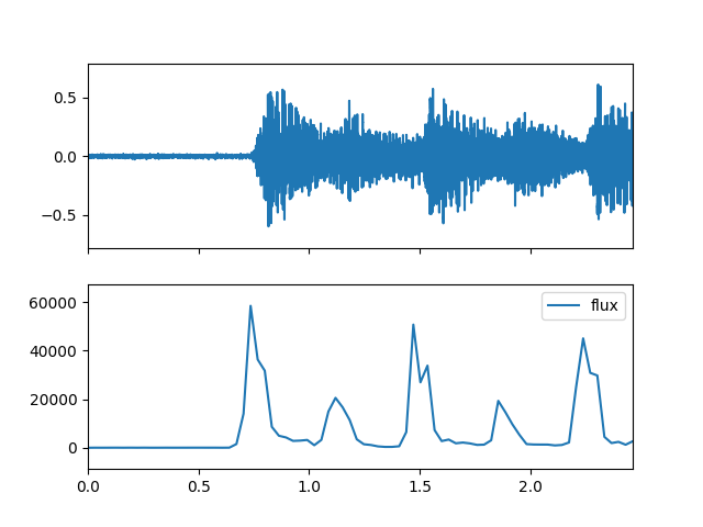
- flux(m_data_arr, step=1, p=2, is_positive=False, is_exp=False, tp=0)
Compute the spectral flux feature.
\(\qquad flux(t)=\left( \sum_{k=b_1}^{b_2} |s_k(t)-s_k(t-1) |^{p} \right)^{\frac{1}{p}}\)
\(b_1\) and \(b_2\): the frequency band bin boundaries
\(s_k\): the spectrum value, which can be magnitude spectrum or power spectrum
In general \(s_k(t) \geq s_k(t-1)\) participate in the calculation
- Parameters
- m_data_arr: np.ndarray [shape=(…, fre, time)]
Spectrogram data.
- step: int
Compute time axis steps, like 1/2/3/…
- p: int, 1 or 2
norm: 1 abs; 2 pow
- is_positive: bool
Whether to set negative numbers to 0
- is_exp: bool
Whether to exp
- tp: int, 0 or 1
0 sum 1 mean
- Returns
- flux: np.ndarray [shape=(…, time)]
flux frequency for each time
Examples
Read chord audio data
>>> import audioflux as af
>>> audio_path = af.utils.sample_path('guitar_chord1')
>>> audio_arr, sr = af.read(audio_path)
Create BFT-Linear object and extract spectrogram
>>> from audioflux.type import SpectralFilterBankScaleType, SpectralDataType
>>> import numpy as np
>>> bft_obj = af.BFT(num=2049, samplate=sr, radix2_exp=12, slide_length=1024,
>>>                data_type=SpectralDataType.MAG,
>>>                scale_type=SpectralFilterBankScaleType.LINEAR)
>>> spec_arr = bft_obj.bft(audio_arr)
>>> spec_arr = np.abs(spec_arr)
Create Spectral object and extract flux feature
>>> spectral_obj = af.Spectral(num=bft_obj.num,
>>>                            fre_band_arr=bft_obj.get_fre_band_arr())
>>> n_time = spec_arr.shape[-1]  # Or use bft_obj.cal_time_length(audio_arr.shape[-1])
>>> spectral_obj.set_time_length(n_time)
>>> flux_arr = spectral_obj.flux(spec_arr)
Display plot
>>> import matplotlib.pyplot as plt
>>> from audioflux.display import fill_plot, fill_wave
>>> fig, ax = plt.subplots(nrows=2, sharex=True)
>>> fill_wave(audio_arr, samplate=sr, axes=ax[0])
>>> times = np.arange(0, len(flux_arr)) * (bft_obj.slide_length / bft_obj.samplate)
>>> fill_plot(times, flux_arr, axes=ax[1], label='flux')
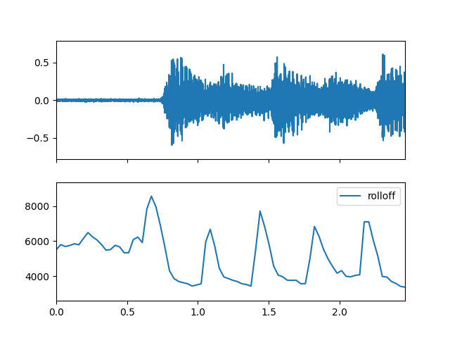
- rolloff(m_data_arr, threshold=0.95)
Compute the spectral rolloff feature.
\(\qquad \sum_{k=b_1}^{i}|s_k| \geq \eta \sum_{k=b_1}^{b_2}s_k\)
\(b_1\) and \(b_2\): the frequency band bin boundaries
\(s_k\): the spectrum value, which can be magnitude spectrum or power spectrum
\(\eta \in (0,1)\), generally take 0.95 or 0.85, satisfy the condition \(i\) get \(f_i\) rolloff frequency
- Parameters
- m_data_arr: np.ndarray [shape=(…, fre, time)]
Spectrogram data.
- threshold: float, [0,1]
rolloff threshold. Generally take 0.95 or 0.85.
- Returns
- rolloff: np.ndarray [shape=(…, time)]
rolloff frequency for each time
Examples
Read chord audio data
>>> import audioflux as af
>>> audio_path = af.utils.sample_path('guitar_chord1')
>>> audio_arr, sr = af.read(audio_path)
Create BFT-Linear object and extract spectrogram
>>> from audioflux.type import SpectralFilterBankScaleType, SpectralDataType
>>> import numpy as np
>>> bft_obj = af.BFT(num=2049, samplate=sr, radix2_exp=12, slide_length=1024,
>>>                data_type=SpectralDataType.MAG,
>>>                scale_type=SpectralFilterBankScaleType.LINEAR)
>>> spec_arr = bft_obj.bft(audio_arr)
>>> spec_arr = np.abs(spec_arr)
Create Spectral object and extract rolloff feature
>>> spectral_obj = af.Spectral(num=bft_obj.num,
>>>                            fre_band_arr=bft_obj.get_fre_band_arr())
>>> n_time = spec_arr.shape[-1]  # Or use bft_obj.cal_time_length(audio_arr.shape[-1])
>>> spectral_obj.set_time_length(n_time)
>>> rolloff_arr = spectral_obj.rolloff(spec_arr)
Display plot
>>> import matplotlib.pyplot as plt
>>> from audioflux.display import fill_plot, fill_wave
>>> fig, ax = plt.subplots(nrows=2, sharex=True)
>>> fill_wave(audio_arr, samplate=sr, axes=ax[0])
>>> times = np.arange(0, len(rolloff_arr)) * (bft_obj.slide_length / bft_obj.samplate)
>>> fill_plot(times, rolloff_arr, axes=ax[1], label='rolloff')
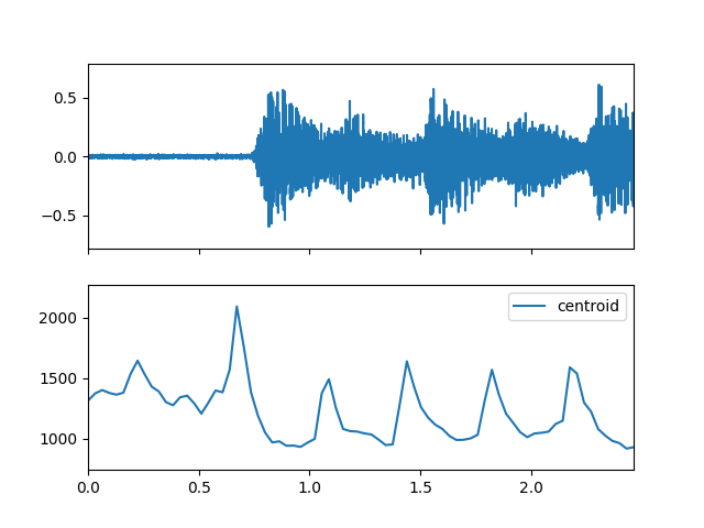
- centroid(m_data_arr)
Compute the spectral centroid feature.
\(\qquad \mu_1=\frac{\sum_{ k=b_1 }^{b_2} f_ks_k } {\sum_{k=b_1}^{b_2} s_k }\)
\(b_1\) and \(b_2\): the frequency band bin boundaries
\(f_k\) is in Hz
\(s_k\): the spectrum value, which can be magnitude spectrum or power spectrum
- Parameters
- m_data_arr: np.ndarray [shape=(…, fre, time)]
Spectrogram data.
- Returns
- centroid: np.ndarray [shape=(…, time)]
centroid frequency for each time
Examples
Read chord audio data
>>> import audioflux as af
>>> audio_path = af.utils.sample_path('guitar_chord1')
>>> audio_arr, sr = af.read(audio_path)
Create BFT-Linear object and extract spectrogram
>>> from audioflux.type import SpectralFilterBankScaleType, SpectralDataType
>>> import numpy as np
>>> bft_obj = af.BFT(num=2049, samplate=sr, radix2_exp=12, slide_length=1024,
>>>                data_type=SpectralDataType.MAG,
>>>                scale_type=SpectralFilterBankScaleType.LINEAR)
>>> spec_arr = bft_obj.bft(audio_arr)
>>> spec_arr = np.abs(spec_arr)
Create Spectral object and extract centroid feature
>>> spectral_obj = af.Spectral(num=bft_obj.num,
>>>                            fre_band_arr=bft_obj.get_fre_band_arr())
>>> n_time = spec_arr.shape[-1]  # Or use bft_obj.cal_time_length(audio_arr.shape[-1])
>>> spectral_obj.set_time_length(n_time)
>>> centroid_arr = spectral_obj.centroid(spec_arr)
Display plot
>>> import matplotlib.pyplot as plt
>>> from audioflux.display import fill_plot, fill_wave
>>> fig, ax = plt.subplots(nrows=2, sharex=True)
>>> fill_wave(audio_arr, samplate=sr, axes=ax[0])
>>> times = np.arange(0, len(centroid_arr)) * (bft_obj.slide_length / bft_obj.samplate)
>>> fill_plot(times, centroid_arr, axes=ax[1], label='centroid')
- spread(m_data_arr)
Compute the spectral spread feature.
\(\qquad \mu_2=\sqrt{\frac{\sum_{ k=b_1 }^{b_2} (f_k-\mu_1)^2 s_k } {\sum_{k=b_1}^{b_2} s_k } }\)
\(b_1\) and \(b_2\): the frequency band bin boundaries
\(f_k\) is in Hz
\(s_k\): the spectrum value, which can be magnitude spectrum or power spectrum
\(u_1\):
Spectral.centroid
- Parameters
- m_data_arr: np.ndarray [shape=(…, fre, time)]
Spectrogram data.
- Returns
- spread: np.ndarray [shape=(…, time)]
spread frequency for each time
Examples
Read chord audio data
>>> import audioflux as af
>>> audio_path = af.utils.sample_path('guitar_chord1')
>>> audio_arr, sr = af.read(audio_path)
Create BFT-Linear object and extract spectrogram
>>> from audioflux.type import SpectralFilterBankScaleType, SpectralDataType
>>> import numpy as np
>>> bft_obj = af.BFT(num=2049, samplate=sr, radix2_exp=12, slide_length=1024,
>>>                data_type=SpectralDataType.MAG,
>>>                scale_type=SpectralFilterBankScaleType.LINEAR)
>>> spec_arr = bft_obj.bft(audio_arr)
>>> spec_arr = np.abs(spec_arr)
Create Spectral object and extract spread feature
>>> spectral_obj = af.Spectral(num=bft_obj.num,
>>>                            fre_band_arr=bft_obj.get_fre_band_arr())
>>> n_time = spec_arr.shape[-1]  # Or use bft_obj.cal_time_length(audio_arr.shape[-1])
>>> spectral_obj.set_time_length(n_time)
>>> spread_arr = spectral_obj.spread(spec_arr)
Display plot
>>> import matplotlib.pyplot as plt
>>> from audioflux.display import fill_plot, fill_wave
>>> fig, ax = plt.subplots(nrows=2, sharex=True)
>>> fill_wave(audio_arr, samplate=sr, axes=ax[0])
>>> times = np.arange(0, len(spread_arr)) * (bft_obj.slide_length / bft_obj.samplate)
>>> fill_plot(times, spread_arr, axes=ax[1], label='spread')

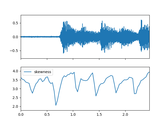
- skewness(m_data_arr)
Compute the spectral skewness feature.
\(\qquad \mu_3=\frac{\sum_{ k=b_1 }^{b_2} (f_k-\mu_1)^3 s_k } {(\mu_2)^3 \sum_{k=b_1}^{b_2} s_k }\)
\(b_1\) and \(b_2\): the frequency band bin boundaries
\(f_k\) is in Hz
\(s_k\): the spectrum value, which can be magnitude spectrum or power spectrum
\(u_1\):
Spectral.centroid\(u_2\):
Spectral.spread
- Parameters
- m_data_arr: np.ndarray [shape=(…, fre, time)]
Spectrogram data.
- Returns
- skewness: np.ndarray [shape=(…, time)]
skewness frequency for each time
Examples
Read chord audio data
>>> import audioflux as af
>>> audio_path = af.utils.sample_path('guitar_chord1')
>>> audio_arr, sr = af.read(audio_path)
Create BFT-Linear object and extract spectrogram
>>> from audioflux.type import SpectralFilterBankScaleType, SpectralDataType
>>> import numpy as np
>>> bft_obj = af.BFT(num=2049, samplate=sr, radix2_exp=12, slide_length=1024,
>>>                data_type=SpectralDataType.MAG,
>>>                scale_type=SpectralFilterBankScaleType.LINEAR)
>>> spec_arr = bft_obj.bft(audio_arr)
>>> spec_arr = np.abs(spec_arr)
Create Spectral object and extract skewness feature
>>> spectral_obj = af.Spectral(num=bft_obj.num,
>>>                            fre_band_arr=bft_obj.get_fre_band_arr())
>>> n_time = spec_arr.shape[-1]  # Or use bft_obj.cal_time_length(audio_arr.shape[-1])
>>> spectral_obj.set_time_length(n_time)
>>> skewness_arr = spectral_obj.skewness(spec_arr)
Display plot
>>> import matplotlib.pyplot as plt
>>> from audioflux.display import fill_plot, fill_wave
>>> fig, ax = plt.subplots(nrows=2, sharex=True)
>>> fill_wave(audio_arr, samplate=sr, axes=ax[0])
>>> times = np.arange(0, len(skewness_arr)) * (bft_obj.slide_length / bft_obj.samplate)
>>> fill_plot(times, skewness_arr, axes=ax[1], label='skewness')
- kurtosis(m_data_arr)
Compute the spectral kurtosis feature.
\(\qquad \mu_4=\frac{\sum_{ k=b_1 }^{b_2} (f_k-\mu_1)^4 s_k } {(\mu_2)^4 \sum_{k=b_1}^{b_2} s_k }\)
\(b_1\) and \(b_2\): the frequency band bin boundaries
\(f_k\) is in Hz
\(s_k\): the spectrum value, which can be magnitude spectrum or power spectrum
\(u_1\):
Spectral.centroid\(u_2\):
Spectral.spread
- Parameters
- m_data_arr: np.ndarray [shape=(…, fre, time)]
Spectrogram data.
- Returns
- kurtosis: np.ndarray [shape=(…, time)]
kurtosis frequency for each time
Examples
Read chord audio data
>>> import audioflux as af
>>> audio_path = af.utils.sample_path('guitar_chord1')
>>> audio_arr, sr = af.read(audio_path)
Create BFT-Linear object and extract spectrogram
>>> from audioflux.type import SpectralFilterBankScaleType, SpectralDataType
>>> import numpy as np
>>> bft_obj = af.BFT(num=2049, samplate=sr, radix2_exp=12, slide_length=1024,
>>>                data_type=SpectralDataType.MAG,
>>>                scale_type=SpectralFilterBankScaleType.LINEAR)
>>> spec_arr = bft_obj.bft(audio_arr)
>>> spec_arr = np.abs(spec_arr)
Create Spectral object and extract kurtosis feature
>>> spectral_obj = af.Spectral(num=bft_obj.num,
>>>                            fre_band_arr=bft_obj.get_fre_band_arr())
>>> n_time = spec_arr.shape[-1]  # Or use bft_obj.cal_time_length(audio_arr.shape[-1])
>>> spectral_obj.set_time_length(n_time)
>>> kurtosis_arr = spectral_obj.kurtosis(spec_arr)
Display plot
>>> import matplotlib.pyplot as plt
>>> from audioflux.display import fill_plot, fill_wave
>>> fig, ax = plt.subplots(nrows=2, sharex=True)
>>> fill_wave(audio_arr, samplate=sr, axes=ax[0])
>>> times = np.arange(0, len(kurtosis_arr)) * (bft_obj.slide_length / bft_obj.samplate)
>>> fill_plot(times, kurtosis_arr, axes=ax[1], label='kurtosis')

- entropy(m_data_arr, is_norm=False)
Compute the spectral entropy feature.
Set: \(p_k=\frac{s_k}{\sum_{k=b_1}^{b_2}s_k}\)
\(\qquad entropy1= \frac{-\sum_{ k=b_1 }^{b_2} p_k \log(p_k)} {\log(b_2-b_1)}\)
Or
\(\qquad entropy2= {-\sum_{ k=b_1 }^{b_2} p_k \log(p_k)}\)
\(b_1\) and \(b_2\): the frequency band bin boundaries
\(s_k\): the spectrum value, which can be magnitude spectrum or power spectrum
- Parameters
- m_data_arr: np.ndarray [shape=(…, fre, time)]
Spectrogram data.
- is_norm: bool
Whether to norm
- Returns
- entropy: np.ndarray [shape=(…, time)]
entropy frequency for each time
Examples
Read chord audio data
>>> import audioflux as af
>>> audio_path = af.utils.sample_path('guitar_chord1')
>>> audio_arr, sr = af.read(audio_path)
Create BFT-Linear object and extract spectrogram
>>> from audioflux.type import SpectralFilterBankScaleType, SpectralDataType
>>> import numpy as np
>>> bft_obj = af.BFT(num=2049, samplate=sr, radix2_exp=12, slide_length=1024,
>>>                data_type=SpectralDataType.MAG,
>>>                scale_type=SpectralFilterBankScaleType.LINEAR)
>>> spec_arr = bft_obj.bft(audio_arr)
>>> spec_arr = np.abs(spec_arr)
Create Spectral object and extract entropy feature
>>> spectral_obj = af.Spectral(num=bft_obj.num,
>>>                            fre_band_arr=bft_obj.get_fre_band_arr())
>>> n_time = spec_arr.shape[-1]  # Or use bft_obj.cal_time_length(audio_arr.shape[-1])
>>> spectral_obj.set_time_length(n_time)
>>> entropy_arr = spectral_obj.entropy(spec_arr)
Display plot
>>> import matplotlib.pyplot as plt
>>> from audioflux.display import fill_plot, fill_wave
>>> fig, ax = plt.subplots(nrows=2, sharex=True)
>>> fill_wave(audio_arr, samplate=sr, axes=ax[0])
>>> times = np.arange(0, len(entropy_arr)) * (bft_obj.slide_length / bft_obj.samplate)
>>> fill_plot(times, entropy_arr, axes=ax[1], label='entropy')

- crest(m_data_arr)
Compute the spectral crest feature.
\(\qquad crest =\frac{max(s_{k\in_{[b_1,b_2]} }) } {\frac{1}{b_2-b_1} \sum_{ k=b_1 }^{b_2} s_k}\)
\(b_1\) and \(b_2\): the frequency band bin boundaries
\(s_k\): the spectrum value, which can be magnitude spectrum or power spectrum
- Parameters
- m_data_arr: np.ndarray [shape=(…, fre, time)]
Spectrogram data.
- Returns
- crest: np.ndarray [shape=(…, time)]
crest frequency for each time
Examples
Read chord audio data
>>> import audioflux as af
>>> audio_path = af.utils.sample_path('guitar_chord1')
>>> audio_arr, sr = af.read(audio_path)
Create BFT-Linear object and extract spectrogram
>>> from audioflux.type import SpectralFilterBankScaleType, SpectralDataType
>>> import numpy as np
>>> bft_obj = af.BFT(num=2049, samplate=sr, radix2_exp=12, slide_length=1024,
>>>                data_type=SpectralDataType.MAG,
>>>                scale_type=SpectralFilterBankScaleType.LINEAR)
>>> spec_arr = bft_obj.bft(audio_arr)
>>> spec_arr = np.abs(spec_arr)
Create Spectral object and extract crest feature
>>> spectral_obj = af.Spectral(num=bft_obj.num,
>>>                            fre_band_arr=bft_obj.get_fre_band_arr())
>>> n_time = spec_arr.shape[-1]  # Or use bft_obj.cal_time_length(audio_arr.shape[-1])
>>> spectral_obj.set_time_length(n_time)
>>> crest_arr = spectral_obj.crest(spec_arr)
Display plot
>>> import matplotlib.pyplot as plt
>>> from audioflux.display import fill_plot, fill_wave
>>> fig, ax = plt.subplots(nrows=2, sharex=True)
>>> fill_wave(audio_arr, samplate=sr, axes=ax[0])
>>> times = np.arange(0, len(crest_arr)) * (bft_obj.slide_length / bft_obj.samplate)
>>> fill_plot(times, crest_arr, axes=ax[1], label='crest')

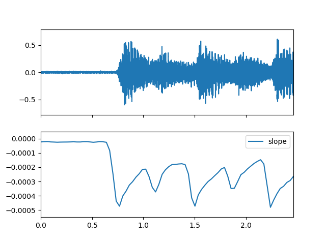
- slope(m_data_arr)
Compute the spectral slope feature.
\(\qquad slope=\frac{ \sum_{k=b_1}^{b_2}(f_k-\mu_f)(s_k-\mu_s) } { \sum_{k=b_1}^{b_2}(f_k-\mu_f)^2 }\)
\(b_1\) and \(b_2\): the frequency band bin boundaries
\(f_k\) is in Hz
\(s_k\): the spectrum value, which can be magnitude spectrum or power spectrum
\(\mu_f\): average frequency value
\(\mu_s\): average spectral value
- Parameters
- m_data_arr: np.ndarray [shape=(…, fre, time)]
Spectrogram data.
- Returns
- slope: np.ndarray [shape=(…, time)]
slope frequency for each time
Examples
Read chord audio data
>>> import audioflux as af
>>> audio_path = af.utils.sample_path('guitar_chord1')
>>> audio_arr, sr = af.read(audio_path)
Create BFT-Linear object and extract spectrogram
>>> from audioflux.type import SpectralFilterBankScaleType, SpectralDataType
>>> import numpy as np
>>> bft_obj = af.BFT(num=2049, samplate=sr, radix2_exp=12, slide_length=1024,
>>>                data_type=SpectralDataType.MAG,
>>>                scale_type=SpectralFilterBankScaleType.LINEAR)
>>> spec_arr = bft_obj.bft(audio_arr)
>>> spec_arr = np.abs(spec_arr)
Create Spectral object and extract slope feature
>>> spectral_obj = af.Spectral(num=bft_obj.num,
>>>                            fre_band_arr=bft_obj.get_fre_band_arr())
>>> n_time = spec_arr.shape[-1]  # Or use bft_obj.cal_time_length(audio_arr.shape[-1])
>>> spectral_obj.set_time_length(n_time)
>>> slope_arr = spectral_obj.slope(spec_arr)
Display plot
>>> import matplotlib.pyplot as plt
>>> from audioflux.display import fill_plot, fill_wave
>>> fig, ax = plt.subplots(nrows=2, sharex=True)
>>> fill_wave(audio_arr, samplate=sr, axes=ax[0])
>>> times = np.arange(0, len(slope_arr)) * (bft_obj.slide_length / bft_obj.samplate)
>>> fill_plot(times, slope_arr, axes=ax[1], label='slope')
- decrease(m_data_arr)
Compute the spectral decrease feature.
\(\qquad decrease=\frac { \sum_{k=b_1+1}^{b_2} \frac {s_k-s_{b_1}}{k-1} } { \sum_{k=b_1+1}^{b_2} s_k }\)
\(b_1\) and \(b_2\): the frequency band bin boundaries
\(s_k\): the spectrum value, which can be magnitude spectrum or power spectrum
- Parameters
- m_data_arr: np.ndarray [shape=(…, fre, time)]
Spectrogram data.
- Returns
- decrease: np.ndarray [shape=(…, time)]
decrease frequency for each time
Examples
Read chord audio data
>>> import audioflux as af
>>> audio_path = af.utils.sample_path('guitar_chord1')
>>> audio_arr, sr = af.read(audio_path)
Create BFT-Linear object and extract spectrogram
>>> from audioflux.type import SpectralFilterBankScaleType, SpectralDataType
>>> import numpy as np
>>> bft_obj = af.BFT(num=2049, samplate=sr, radix2_exp=12, slide_length=1024,
>>>                data_type=SpectralDataType.MAG,
>>>                scale_type=SpectralFilterBankScaleType.LINEAR)
>>> spec_arr = bft_obj.bft(audio_arr)
>>> spec_arr = np.abs(spec_arr)
Create Spectral object and extract decrease feature
>>> spectral_obj = af.Spectral(num=bft_obj.num,
>>>                            fre_band_arr=bft_obj.get_fre_band_arr())
>>> n_time = spec_arr.shape[-1]  # Or use bft_obj.cal_time_length(audio_arr.shape[-1])
>>> spectral_obj.set_time_length(n_time)
>>> decrease_arr = spectral_obj.decrease(spec_arr)
Display plot
>>> import matplotlib.pyplot as plt
>>> from audioflux.display import fill_plot, fill_wave
>>> fig, ax = plt.subplots(nrows=2, sharex=True)
>>> fill_wave(audio_arr, samplate=sr, axes=ax[0])
>>> times = np.arange(0, len(decrease_arr)) * (bft_obj.slide_length / bft_obj.samplate)
>>> fill_plot(times, decrease_arr, axes=ax[1], label='decrease')

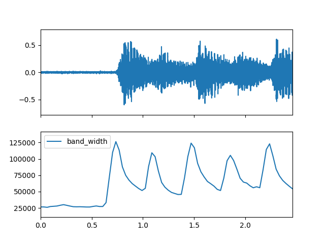
- band_width(m_data_arr, p=2)
Compute the spectral band_width feature.
\(\qquad bandwidth=\left(\sum_{k=b_1}^{b_2} s_k(f_k-centroid)^p \right)^{\frac{1}{p}}\)
\(b_1\) and \(b_2\): the frequency band bin boundaries
\(f_k\) is in Hz
\(s_k\): the spectrum value, which can be magnitude spectrum or power spectrum
centroid:
Spectral.centroid
- Parameters
- m_data_arr: np.ndarray [shape=(…, fre, time)]
Spectrogram data.
- p: int, 1 or 2
norm: 1 abs; 2 pow
- Returns
- band_width: np.ndarray [shape=(…, time)]
band_width frequency for each time
Examples
Read chord audio data
>>> import audioflux as af
>>> audio_path = af.utils.sample_path('guitar_chord1')
>>> audio_arr, sr = af.read(audio_path)
Create BFT-Linear object and extract spectrogram
>>> from audioflux.type import SpectralFilterBankScaleType, SpectralDataType
>>> import numpy as np
>>> bft_obj = af.BFT(num=2049, samplate=sr, radix2_exp=12, slide_length=1024,
>>>                data_type=SpectralDataType.MAG,
>>>                scale_type=SpectralFilterBankScaleType.LINEAR)
>>> spec_arr = bft_obj.bft(audio_arr)
>>> spec_arr = np.abs(spec_arr)
Create Spectral object and extract band_width feature
>>> spectral_obj = af.Spectral(num=bft_obj.num,
>>>                            fre_band_arr=bft_obj.get_fre_band_arr())
>>> n_time = spec_arr.shape[-1]  # Or use bft_obj.cal_time_length(audio_arr.shape[-1])
>>> spectral_obj.set_time_length(n_time)
>>> band_width_arr = spectral_obj.band_width(spec_arr)
Display plot
>>> import matplotlib.pyplot as plt
>>> from audioflux.display import fill_plot, fill_wave
>>> fig, ax = plt.subplots(nrows=2, sharex=True)
>>> fill_wave(audio_arr, samplate=sr, axes=ax[0])
>>> times = np.arange(0, len(band_width_arr)) * (bft_obj.slide_length / bft_obj.samplate)
>>> fill_plot(times, band_width_arr, axes=ax[1], label='band_width')
- rms(m_data_arr)
Compute the spectral rms feature.
\(\qquad rms=\sqrt{ \frac{1}{N} \sum_{n=1}^N x^2[n] }=\sqrt {\frac{1}{N^2}\sum_{m=1}^N |X[m]|^2 }\)
- Parameters
- m_data_arr: np.ndarray [shape=(…, fre, time)]
Spectrogram data.
- Returns
- rms: np.ndarray [shape=(…. time)]
rms frequency for each time
Examples
Read chord audio data
>>> import audioflux as af
>>> audio_path = af.utils.sample_path('guitar_chord1')
>>> audio_arr, sr = af.read(audio_path)
Create BFT-Linear object and extract spectrogram
>>> from audioflux.type import SpectralFilterBankScaleType, SpectralDataType
>>> import numpy as np
>>> bft_obj = af.BFT(num=2049, samplate=sr, radix2_exp=12, slide_length=1024,
>>>                data_type=SpectralDataType.MAG,
>>>                scale_type=SpectralFilterBankScaleType.LINEAR)
>>> spec_arr = bft_obj.bft(audio_arr)
>>> spec_arr = np.abs(spec_arr)
Create Spectral object and extract rms feature
>>> spectral_obj = af.Spectral(num=bft_obj.num,
>>>                            fre_band_arr=bft_obj.get_fre_band_arr())
>>> n_time = spec_arr.shape[-1]  # Or use bft_obj.cal_time_length(audio_arr.shape[-1])
>>> spectral_obj.set_time_length(n_time)
>>> rms_arr = spectral_obj.rms(spec_arr)
Display plot
>>> import matplotlib.pyplot as plt
>>> from audioflux.display import fill_plot, fill_wave
>>> fig, ax = plt.subplots(nrows=2, sharex=True)
>>> fill_wave(audio_arr, samplate=sr, axes=ax[0])
>>> times = np.arange(0, len(rms_arr)) * (bft_obj.slide_length / bft_obj.samplate)
>>> fill_plot(times, rms_arr, axes=ax[1], label='rms')

- energy(m_data_arr, is_log=False, gamma=10.0)
Compute the spectral energy feature.
\(\qquad energy=\sum_{n=1}^N x^2[n] =\frac{1}{N}\sum_{m=1}^N |X[m]|^2\)
- Parameters
- m_data_arr: np.ndarray [shape=(…, fre, time)]
Spectrogram data.
- is_log: bool
Whether to log
- gamma: float
energy gamma value.
- Returns
- energy: np.ndarray [shape=(…, time)]
energy frequency for each time
Examples
Read chord audio data
>>> import audioflux as af
>>> audio_path = af.utils.sample_path('guitar_chord1')
>>> audio_arr, sr = af.read(audio_path)
Create BFT-Linear object and extract spectrogram
>>> from audioflux.type import SpectralFilterBankScaleType, SpectralDataType
>>> import numpy as np
>>> bft_obj = af.BFT(num=2049, samplate=sr, radix2_exp=12, slide_length=1024,
>>>                data_type=SpectralDataType.MAG,
>>>                scale_type=SpectralFilterBankScaleType.LINEAR)
>>> spec_arr = bft_obj.bft(audio_arr)
>>> spec_arr = np.abs(spec_arr)
Create Spectral object and extract energy feature
>>> spectral_obj = af.Spectral(num=bft_obj.num,
>>>                            fre_band_arr=bft_obj.get_fre_band_arr())
>>> n_time = spec_arr.shape[-1]  # Or use bft_obj.cal_time_length(audio_arr.shape[-1])
>>> spectral_obj.set_time_length(n_time)
>>> energy_arr = spectral_obj.energy(spec_arr)
Display plot
>>> import matplotlib.pyplot as plt
>>> from audioflux.display import fill_plot, fill_wave
>>> fig, ax = plt.subplots(nrows=2, sharex=True)
>>> fill_wave(audio_arr, samplate=sr, axes=ax[0])
>>> times = np.arange(0, len(energy_arr)) * (bft_obj.slide_length / bft_obj.samplate)
>>> fill_plot(times, energy_arr, axes=ax[1], label='energy')

- hfc(m_data_arr)
Compute the spectral hfc feature.
\(\qquad hfc(t)=\frac{\sum_{k=b_1}^{b_2} s_k(t)k }{b_2-b_1+1}\)
\(b_1\) and \(b_2\): the frequency band bin boundaries
\(s_k\): the spectrum value, which can be magnitude spectrum or power spectrum
- Parameters
- m_data_arr: np.ndarray [shape=(…, fre, time)]
Spectrogram data.
- Returns
- hfc: np.ndarray [shape=(…, time)]
hfc frequency for each time
Examples
Read chord audio data
>>> import audioflux as af
>>> audio_path = af.utils.sample_path('guitar_chord1')
>>> audio_arr, sr = af.read(audio_path)
Create BFT-Linear object and extract spectrogram
>>> from audioflux.type import SpectralFilterBankScaleType, SpectralDataType
>>> import numpy as np
>>> bft_obj = af.BFT(num=2049, samplate=sr, radix2_exp=12, slide_length=1024,
>>>                data_type=SpectralDataType.MAG,
>>>                scale_type=SpectralFilterBankScaleType.LINEAR)
>>> spec_arr = bft_obj.bft(audio_arr)
>>> spec_arr = np.abs(spec_arr)
Create Spectral object and extract hfc feature
>>> spectral_obj = af.Spectral(num=bft_obj.num,
>>>                            fre_band_arr=bft_obj.get_fre_band_arr())
>>> n_time = spec_arr.shape[-1]  # Or use bft_obj.cal_time_length(audio_arr.shape[-1])
>>> spectral_obj.set_time_length(n_time)
>>> hfc_arr = spectral_obj.hfc(spec_arr)
Display plot
>>> import matplotlib.pyplot as plt
>>> from audioflux.display import fill_plot, fill_wave
>>> fig, ax = plt.subplots(nrows=2, sharex=True)
>>> fill_wave(audio_arr, samplate=sr, axes=ax[0])
>>> times = np.arange(0, len(hfc_arr)) * (bft_obj.slide_length / bft_obj.samplate)
>>> fill_plot(times, hfc_arr, axes=ax[1], label='hfc')

- sd(m_data_arr, step=1, is_positive=False)
Compute the spectral sd feature.
\(\qquad sd(t)=flux(t)\)
satisfies the calculation of \(s_k(t) \ge s_k(t-1)\), \(p=2\),the result is not \(1/p\)
\(s_k\): the spectrum value, which can be magnitude spectrum or power spectrum
flux:
Spectral.flux
- Parameters
- m_data_arr: np.ndarray [shape=(…, fre, time)]
Spectrogram data.
- step: int
Compute time axis steps, like 1/2/3/…
- is_positive: bool
Whether to set negative numbers to 0
- Returns
- sd: np.ndarray [shape=(…, time)]
sd frequency for each time
Examples
Read chord audio data
>>> import audioflux as af
>>> audio_path = af.utils.sample_path('guitar_chord1')
>>> audio_arr, sr = af.read(audio_path)
Create BFT-Linear object and extract spectrogram
>>> from audioflux.type import SpectralFilterBankScaleType, SpectralDataType
>>> import numpy as np
>>> bft_obj = af.BFT(num=2049, samplate=sr, radix2_exp=12, slide_length=1024,
>>>                data_type=SpectralDataType.MAG,
>>>                scale_type=SpectralFilterBankScaleType.LINEAR)
>>> spec_arr = bft_obj.bft(audio_arr)
>>> spec_arr = np.abs(spec_arr)
Create Spectral object and extract sd feature
>>> spectral_obj = af.Spectral(num=bft_obj.num,
>>>                            fre_band_arr=bft_obj.get_fre_band_arr())
>>> n_time = spec_arr.shape[-1]  # Or use bft_obj.cal_time_length(audio_arr.shape[-1])
>>> spectral_obj.set_time_length(n_time)
>>> sd_arr = spectral_obj.sd(spec_arr)
Display plot
>>> import matplotlib.pyplot as plt
>>> from audioflux.display import fill_plot, fill_wave
>>> fig, ax = plt.subplots(nrows=2, sharex=True)
>>> fill_wave(audio_arr, samplate=sr, axes=ax[0])
>>> times = np.arange(0, len(sd_arr)) * (bft_obj.slide_length / bft_obj.samplate)
>>> fill_plot(times, sd_arr, axes=ax[1], label='sd')

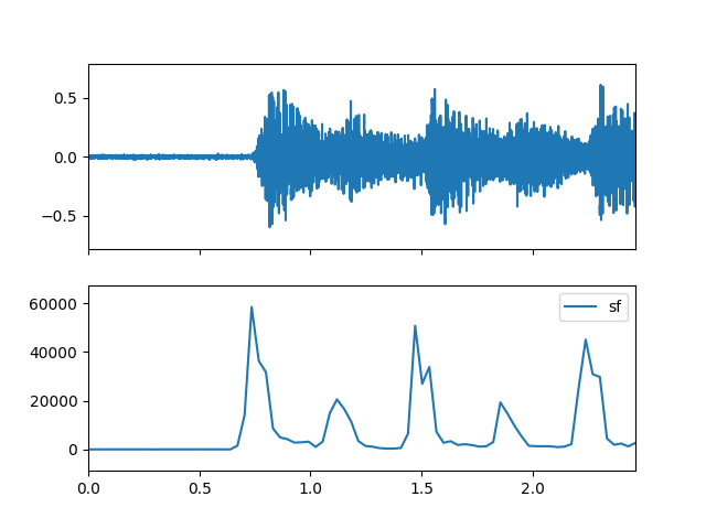
- sf(m_data_arr, step=1, is_positive=False)
Compute the spectral sf feature.
\(\qquad sf(t)=flux(t)\)
satisfies the calculation of \(s_k(t) \ge s_k(t-1)\), \(p=1\)
\(s_k\): the spectrum value, which can be magnitude spectrum or power spectrum
flux:
Spectral.flux
- Parameters
- m_data_arr: np.ndarray [shape=(…, fre, time)]
Spectrogram data.
- step: int
Compute time axis steps, like 1/2/3/…
- is_positive: bool
Whether to set negative numbers to 0
- Returns
- sf: np.ndarray [shape=(…, time)]
sf frequency for each time
Examples
Read chord audio data
>>> import audioflux as af
>>> audio_path = af.utils.sample_path('guitar_chord1')
>>> audio_arr, sr = af.read(audio_path)
Create BFT-Linear object and extract spectrogram
>>> from audioflux.type import SpectralFilterBankScaleType, SpectralDataType
>>> import numpy as np
>>> bft_obj = af.BFT(num=2049, samplate=sr, radix2_exp=12, slide_length=1024,
>>>                data_type=SpectralDataType.MAG,
>>>                scale_type=SpectralFilterBankScaleType.LINEAR)
>>> spec_arr = bft_obj.bft(audio_arr)
>>> spec_arr = np.abs(spec_arr)
Create Spectral object and extract sf feature
>>> spectral_obj = af.Spectral(num=bft_obj.num,
>>>                            fre_band_arr=bft_obj.get_fre_band_arr())
>>> n_time = spec_arr.shape[-1]  # Or use bft_obj.cal_time_length(audio_arr.shape[-1])
>>> spectral_obj.set_time_length(n_time)
>>> sf_arr = spectral_obj.sf(spec_arr)
Display plot
>>> import matplotlib.pyplot as plt
>>> from audioflux.display import fill_plot, fill_wave
>>> fig, ax = plt.subplots(nrows=2, sharex=True)
>>> fill_wave(audio_arr, samplate=sr, axes=ax[0])
>>> times = np.arange(0, len(sf_arr)) * (bft_obj.slide_length / bft_obj.samplate)
>>> fill_plot(times, sf_arr, axes=ax[1], label='sf')
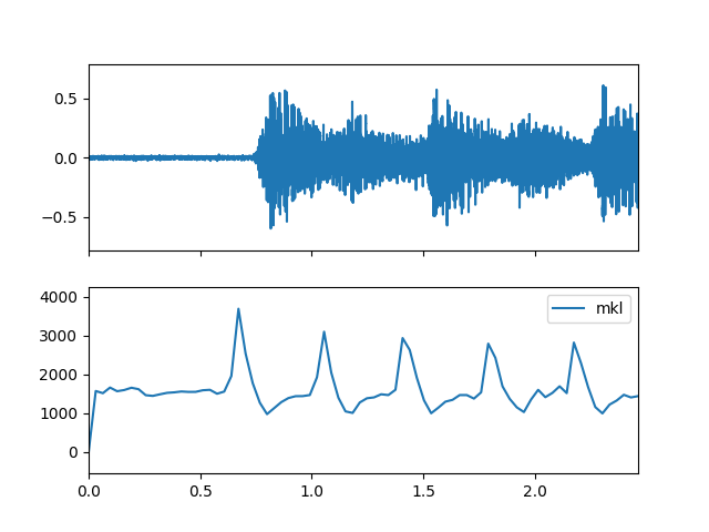
- mkl(m_data_arr, tp=0)
Compute the spectral mkl feature.
\(\qquad mkl(t)=\sum_{k=b_1}^{b_2} \log\left(1+ \cfrac {s_k(t)}{s_k(t-1)} \right)\)
\(b_1\) and \(b_2\): the frequency band bin boundaries
\(s_k\): the spectrum value, which can be magnitude spectrum or power spectrum
- Parameters
- m_data_arr: np.ndarray [shape=(…, fre, time)]
Spectrogram data.
- tp: int, 0 or 1
0 sum 1 mean
- Returns
- mkl: np.ndarray [shape=(…, time)]
mkl frequency for each time
Examples
Read chord audio data
>>> import audioflux as af
>>> audio_path = af.utils.sample_path('guitar_chord1')
>>> audio_arr, sr = af.read(audio_path)
Create BFT-Linear object and extract spectrogram
>>> from audioflux.type import SpectralFilterBankScaleType, SpectralDataType
>>> import numpy as np
>>> bft_obj = af.BFT(num=2049, samplate=sr, radix2_exp=12, slide_length=1024,
>>>                data_type=SpectralDataType.MAG,
>>>                scale_type=SpectralFilterBankScaleType.LINEAR)
>>> spec_arr = bft_obj.bft(audio_arr)
>>> spec_arr = np.abs(spec_arr)
Create Spectral object and extract mkl feature
>>> spectral_obj = af.Spectral(num=bft_obj.num,
>>>                            fre_band_arr=bft_obj.get_fre_band_arr())
>>> n_time = spec_arr.shape[-1]  # Or use bft_obj.cal_time_length(audio_arr.shape[-1])
>>> spectral_obj.set_time_length(n_time)
>>> mkl_arr = spectral_obj.mkl(spec_arr)
Display plot
>>> import matplotlib.pyplot as plt
>>> from audioflux.display import fill_plot, fill_wave
>>> fig, ax = plt.subplots(nrows=2, sharex=True)
>>> fill_wave(audio_arr, samplate=sr, axes=ax[0])
>>> times = np.arange(0, len(mkl_arr)) * (bft_obj.slide_length / bft_obj.samplate)
>>> fill_plot(times, mkl_arr, axes=ax[1], label='mkl')
- pd(m_data_arr, m_phase_arr)
Compute the spectral pd feature.
\(\qquad \psi_k(t)\) is set as the phase function of point k at time t.
\(\qquad \psi_k^{\prime}(t)=\psi_k(t)-\psi_k(t-1)\)
\(\qquad \psi_k^{\prime\prime}(t)=\psi_k^{\prime}(t)-\psi_k^{\prime}(t-1) = \psi_k(t)-2\psi_k(t-1)+\psi_k(t-2)\)
\(\qquad pd(t)= \frac {\sum_{k=b_1}^{b_2} \| \psi_k^{\prime\prime}(t) \|} {b_2-b_1+1}\)
\(b_1\) and \(b_2\): the frequency band bin boundaries
- Parameters
- m_data_arr: np.ndarray [shape=(…, fre, time)]
Spectrogram data.
- m_phase_arr: np.ndarray [shape=(…, fre, time)]
Phase data.
- Returns
- pd: np.ndarray [shape=(…, time)]
pd frequency for each time
Examples
Read chord audio data
>>> import audioflux as af
>>> audio_path = af.utils.sample_path('guitar_chord1')
>>> audio_arr, sr = af.read(audio_path)
Create BFT-Linear object and extract spectrogram
>>> from audioflux.type import SpectralFilterBankScaleType, SpectralDataType
>>> import numpy as np
>>> bft_obj = af.BFT(num=2049, samplate=sr, radix2_exp=12, slide_length=1024,
>>>                data_type=SpectralDataType.MAG,
>>>                scale_type=SpectralFilterBankScaleType.LINEAR)
>>> spec_arr = bft_obj.bft(audio_arr)
>>> phase_arr = af.utils.get_phase(spec_arr)
>>> spec_arr = np.abs(spec_arr)
Create Spectral object and extract pd feature
>>> spectral_obj = af.Spectral(num=bft_obj.num,
>>>                            fre_band_arr=bft_obj.get_fre_band_arr())
>>> n_time = spec_arr.shape[-1]  # Or use bft_obj.cal_time_length(audio_arr.shape[-1])
>>> spectral_obj.set_time_length(n_time)
>>> pd_arr = spectral_obj.pd(spec_arr, phase_arr)
- wpd(m_data_arr, m_phase_arr)
Compute the spectral wpd feature.
\(\qquad \psi_k(t)\) is set as the phase function of point k at time t.
\(\qquad \psi_k^{\prime}(t)=\psi_k(t)-\psi_k(t-1)\)
\(\qquad \psi_k^{\prime\prime}(t)=\psi_k^{\prime}(t)-\psi_k^{\prime}(t-1) = \psi_k(t)-2\psi_k(t-1)+\psi_k(t-2)\)
\(\qquad wpd(t)= \frac {\sum_{k=b_1}^{b_2} \| \psi_k^{\prime\prime}(t) \|s_k(t)}{b_2-b_1+1}\)
\(b_1\) and \(b_2\): the frequency band bin boundaries
\(s_k\): the spectrum value, which can be magnitude spectrum or power spectrum
- Parameters
- m_data_arr: np.ndarray [shape=(…, fre, time)]
Spectrogram data.
- m_phase_arr: np.ndarray [shape=(…, fre, time)]
Phase data.
- Returns
- wpd: np.ndarray [shape=(…, time)]
wpd frequency for each time
Examples
Read chord audio data
>>> import audioflux as af
>>> audio_path = af.utils.sample_path('guitar_chord1')
>>> audio_arr, sr = af.read(audio_path)
Create BFT-Linear object and extract spectrogram
>>> from audioflux.type import SpectralFilterBankScaleType, SpectralDataType
>>> import numpy as np
>>> bft_obj = af.BFT(num=2049, samplate=sr, radix2_exp=12, slide_length=1024,
>>>                data_type=SpectralDataType.MAG,
>>>                scale_type=SpectralFilterBankScaleType.LINEAR)
>>> spec_arr = bft_obj.bft(audio_arr)
>>> phase_arr = af.utils.get_phase(spec_arr)
>>> spec_arr = np.abs(spec_arr)
Create Spectral object and extract wpd feature
>>> spectral_obj = af.Spectral(num=bft_obj.num,
>>>                            fre_band_arr=bft_obj.get_fre_band_arr())
>>> n_time = spec_arr.shape[-1]  # Or use bft_obj.cal_time_length(audio_arr.shape[-1])
>>> spectral_obj.set_time_length(n_time)
>>> wpd_arr = spectral_obj.wpd(spec_arr, phase_arr)
Display plot
>>> import matplotlib.pyplot as plt
>>> from audioflux.display import fill_plot, fill_wave
>>> fig, ax = plt.subplots(nrows=2, sharex=True)
>>> fill_wave(audio_arr, samplate=sr, axes=ax[0])
>>> times = np.arange(0, len(wpd_arr)) * (bft_obj.slide_length / bft_obj.samplate)
>>> fill_plot(times, wpd_arr, axes=ax[1], label='wpd')

- nwpd(m_data_arr, m_phase_arr)
Compute the spectral nwpd feature.
\(\qquad nwpd(t)= \frac {wpd} {\mu_s}\)
wpd:
Spectral.wpd\(\mu_s\): the mean of \(s_k(t)\)
\(s_k\): the spectrum value, which can be magnitude spectrum or power spectrum
- Parameters
- m_data_arr: np.ndarray [shape=(…, fre, time)]
Spectrogram data.
- m_phase_arr: np.ndarray [shape=(…, fre, time)]
Phase data.
- Returns
- nwpd: np.ndarray [shape=(…, time)]
nwpd frequency for each time
Examples
Read chord audio data
>>> import audioflux as af
>>> audio_path = af.utils.sample_path('guitar_chord1')
>>> audio_arr, sr = af.read(audio_path)
Create BFT-Linear object and extract spectrogram
>>> from audioflux.type import SpectralFilterBankScaleType, SpectralDataType
>>> import numpy as np
>>> bft_obj = af.BFT(num=2049, samplate=sr, radix2_exp=12, slide_length=1024,
>>>                data_type=SpectralDataType.MAG,
>>>                scale_type=SpectralFilterBankScaleType.LINEAR)
>>> spec_arr = bft_obj.bft(audio_arr)
>>> phase_arr = af.utils.get_phase(spec_arr)
>>> spec_arr = np.abs(spec_arr)
Create Spectral object and extract nwpd feature
>>> spectral_obj = af.Spectral(num=bft_obj.num,
>>>                            fre_band_arr=bft_obj.get_fre_band_arr())
>>> n_time = spec_arr.shape[-1]  # Or use bft_obj.cal_time_length(audio_arr.shape[-1])
>>> spectral_obj.set_time_length(n_time)
>>> nwpd_arr = spectral_obj.nwpd(spec_arr, phase_arr)
- cd(m_data_arr, m_phase_arr)
Compute the spectral cd feature.
\(\qquad \psi_k(t)\) is set as the phase function of point k at time t.
\(\qquad \alpha_k(t)=s_k(t) e^{j(2\psi_k(t)-\psi_k(t-1))}\)
\(\qquad \beta_k(t)=s_k(t) e^{j\psi_k(t)}\)
\(\qquad cd(t)=\sum_{k=b_1}^{b_2} \| \beta_k(t)-\alpha_k(t-1) \|\)
\(b_1\) and \(b_2\): the frequency band bin boundaries
\(s_k\): the spectrum value, which can be magnitude spectrum or power spectrum
- Parameters
- m_data_arr: np.ndarray [shape=(…, fre, time)]
Spectrogram data.
- m_phase_arr: np.ndarray [shape=(…, fre, time)]
Phase data.
- Returns
- cd: np.ndarray [shape=(…, time)]
cd frequency for each time
Examples
Read chord audio data
>>> import audioflux as af
>>> audio_path = af.utils.sample_path('guitar_chord1')
>>> audio_arr, sr = af.read(audio_path)
Create BFT-Linear object and extract spectrogram
>>> from audioflux.type import SpectralFilterBankScaleType, SpectralDataType
>>> import numpy as np
>>> bft_obj = af.BFT(num=2049, samplate=sr, radix2_exp=12, slide_length=1024,
>>>                data_type=SpectralDataType.MAG,
>>>                scale_type=SpectralFilterBankScaleType.LINEAR)
>>> spec_arr = bft_obj.bft(audio_arr)
>>> phase_arr = af.utils.get_phase(spec_arr)
>>> spec_arr = np.abs(spec_arr)
Create Spectral object and extract cd feature
>>> spectral_obj = af.Spectral(num=bft_obj.num,
>>>                            fre_band_arr=bft_obj.get_fre_band_arr())
>>> n_time = spec_arr.shape[-1]  # Or use bft_obj.cal_time_length(audio_arr.shape[-1])
>>> spectral_obj.set_time_length(n_time)
>>> cd_arr = spectral_obj.cd(spec_arr, phase_arr)
Display plot
>>> import matplotlib.pyplot as plt
>>> from audioflux.display import fill_plot, fill_wave
>>> fig, ax = plt.subplots(nrows=2, sharex=True)
>>> fill_wave(audio_arr, samplate=sr, axes=ax[0])
>>> times = np.arange(0, len(cd_arr)) * (bft_obj.slide_length / bft_obj.samplate)
>>> fill_plot(times, cd_arr, axes=ax[1], label='cd')

- rcd(m_data_arr, m_phase_arr)
Compute the spectral rcd feature.
\(\qquad rcd(t)=cd\)
participate in the sum calculation when \(s_k(t) \geq s_k(t-1)\) is satisfied
cd:
Spectral.cd\(s_k\): the spectrum value, which can be magnitude spectrum or power spectrum
- Parameters
- m_data_arr: np.ndarray [shape=(…, fre, time)]
Spectrogram data.
- m_phase_arr: np.ndarray [shape=(…, fre, time)]
Phase data.
- Returns
- rcd: np.ndarray [shape=(…, time)]
rcd frequency for each time
Examples
Read chord audio data
>>> import audioflux as af
>>> audio_path = af.utils.sample_path('guitar_chord1')
>>> audio_arr, sr = af.read(audio_path)
Create BFT-Linear object and extract spectrogram
>>> from audioflux.type import SpectralFilterBankScaleType, SpectralDataType
>>> import numpy as np
>>> bft_obj = af.BFT(num=2049, samplate=sr, radix2_exp=12, slide_length=1024,
>>>                data_type=SpectralDataType.MAG,
>>>                scale_type=SpectralFilterBankScaleType.LINEAR)
>>> spec_arr = bft_obj.bft(audio_arr)
>>> phase_arr = af.utils.get_phase(spec_arr)
>>> spec_arr = np.abs(spec_arr)
Create Spectral object and extract rcd feature
>>> spectral_obj = af.Spectral(num=bft_obj.num,
>>>                            fre_band_arr=bft_obj.get_fre_band_arr())
>>> n_time = spec_arr.shape[-1]  # Or use bft_obj.cal_time_length(audio_arr.shape[-1])
>>> spectral_obj.set_time_length(n_time)
>>> rcd_arr = spectral_obj.rcd(spec_arr, phase_arr)
Display plot
>>> import matplotlib.pyplot as plt
>>> from audioflux.display import fill_plot, fill_wave
>>> fig, ax = plt.subplots(nrows=2, sharex=True)
>>> fill_wave(audio_arr, samplate=sr, axes=ax[0])
>>> times = np.arange(0, len(rcd_arr)) * (bft_obj.slide_length / bft_obj.samplate)
>>> fill_plot(times, rcd_arr, axes=ax[1], label='rcd')

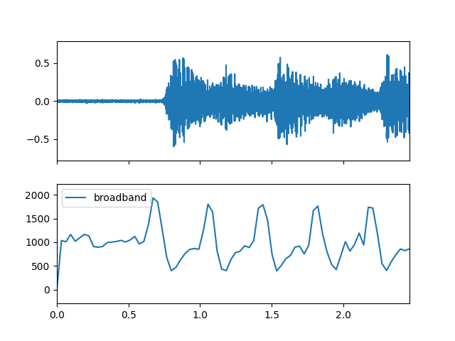
- broadband(m_data_arr, threshold=0)
Compute the spectral broadband feature.
- Parameters
- m_data_arr: np.ndarray [shape=(…, fre, time)]
Spectrogram data.
- threshold: float, [0,1]
broadband threshold
- Returns
- broadband: np.ndarray [shape=(…, time)]
broadband frequency for each time
Examples
Read chord audio data
>>> import audioflux as af
>>> audio_path = af.utils.sample_path('guitar_chord1')
>>> audio_arr, sr = af.read(audio_path)
Create BFT-Linear object and extract spectrogram
>>> from audioflux.type import SpectralFilterBankScaleType, SpectralDataType
>>> import numpy as np
>>> bft_obj = af.BFT(num=2049, samplate=sr, radix2_exp=12, slide_length=1024,
>>>                data_type=SpectralDataType.MAG,
>>>                scale_type=SpectralFilterBankScaleType.LINEAR)
>>> spec_arr = bft_obj.bft(audio_arr)
>>> spec_arr = np.abs(spec_arr)
Create Spectral object and extract broadband feature
>>> spectral_obj = af.Spectral(num=bft_obj.num,
>>>                            fre_band_arr=bft_obj.get_fre_band_arr())
>>> n_time = spec_arr.shape[-1]  # Or use bft_obj.cal_time_length(audio_arr.shape[-1])
>>> spectral_obj.set_time_length(n_time)
>>> broadband_arr = spectral_obj.broadband(spec_arr)
Display plot
>>> import matplotlib.pyplot as plt
>>> from audioflux.display import fill_plot, fill_wave
>>> fig, ax = plt.subplots(nrows=2, sharex=True)
>>> fill_wave(audio_arr, samplate=sr, axes=ax[0])
>>> times = np.arange(0, len(broadband_arr)) * (bft_obj.slide_length / bft_obj.samplate)
>>> fill_plot(times, broadband_arr, axes=ax[1], label='broadband')
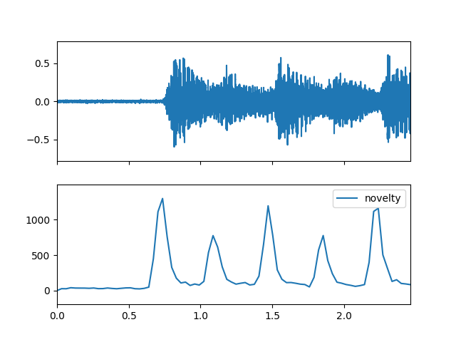
- novelty(m_data_arr, step=1, threshold=0.0, method_type=SpectralNoveltyMethodType.SUB, data_type=SpectralNoveltyDataType.VALUE)
Compute the spectral novelty feature.
- Parameters
- m_data_arr: np.ndarray [shape=(…, fre, time)]
Spectrogram data.
- step: int
Compute time axis steps, like 1/2/3/…
- threshold: float [0,1]
Novelty threshold.
- method_type: SpectralNoveltyMethodType
Novelty method type.
- data_type: SpectralNoveltyDataType
Novelty data type.
- Returns
- novelty: np.ndarray [shape=(…, time)]
Novelty frequency per time step.
Examples
Read chord audio data
>>> import audioflux as af
>>> audio_path = af.utils.sample_path('guitar_chord1')
>>> audio_arr, sr = af.read(audio_path)
Create BFT-Linear object and extract spectrogram
>>> from audioflux.type import SpectralFilterBankScaleType, SpectralDataType
>>> import numpy as np
>>> bft_obj = af.BFT(num=2049, samplate=sr, radix2_exp=12, slide_length=1024,
>>>                data_type=SpectralDataType.MAG,
>>>                scale_type=SpectralFilterBankScaleType.LINEAR)
>>> spec_arr = bft_obj.bft(audio_arr)
>>> spec_arr = np.abs(spec_arr)
Create Spectral object and extract novelty feature
>>> spectral_obj = af.Spectral(num=bft_obj.num,
>>>                            fre_band_arr=bft_obj.get_fre_band_arr())
>>> n_time = spec_arr.shape[-1]  # Or use bft_obj.cal_time_length(audio_arr.shape[-1])
>>> spectral_obj.set_time_length(n_time)
>>> novelty_arr = spectral_obj.novelty(spec_arr)
Display plot
>>> import matplotlib.pyplot as plt
>>> from audioflux.display import fill_plot, fill_wave
>>> fig, ax = plt.subplots(nrows=2, sharex=True)
>>> fill_wave(audio_arr, samplate=sr, axes=ax[0])
>>> times = np.arange(0, len(novelty_arr)) * (bft_obj.slide_length / bft_obj.samplate)
>>> fill_plot(times, novelty_arr, axes=ax[1], label='novelty')
- eef(m_data_arr, is_norm=False)
Compute the spectral eef feature.
\(\qquad p_k=\frac{s_k}{\sum_{k=b_1}^{b_2}s_k}\)
\(\qquad entropy2= {-\sum_{ k=b_1 }^{b_2} p_k \log(p_k)}\)
\(\qquad eef=\sqrt{ 1+| energy\times entropy2| }\)
energy:
Spectral.energy\(b_1\) and \(b_2\): the frequency band bin boundaries
\(s_k\): the spectrum value, which can be magnitude spectrum or power spectrum
- Parameters
- m_data_arr: np.ndarray [shape=(…, fre, time)]
Spectrogram data.
- is_norm: bool
Whether to norm
- Returns
- eef: np.ndarray [shape=(…, time)]
eef frequency for each time
Examples
Read chord audio data
>>> import audioflux as af
>>> audio_path = af.utils.sample_path('guitar_chord1')
>>> audio_arr, sr = af.read(audio_path)
Create BFT-Linear object and extract spectrogram
>>> from audioflux.type import SpectralFilterBankScaleType, SpectralDataType
>>> import numpy as np
>>> bft_obj = af.BFT(num=2049, samplate=sr, radix2_exp=12, slide_length=1024,
>>>                data_type=SpectralDataType.MAG,
>>>                scale_type=SpectralFilterBankScaleType.LINEAR)
>>> spec_arr = bft_obj.bft(audio_arr)
>>> spec_arr = np.abs(spec_arr)
Create Spectral object and extract eef feature
>>> spectral_obj = af.Spectral(num=bft_obj.num,
>>>                            fre_band_arr=bft_obj.get_fre_band_arr())
>>> n_time = spec_arr.shape[-1]  # Or use bft_obj.cal_time_length(audio_arr.shape[-1])
>>> spectral_obj.set_time_length(n_time)
>>> eef_arr = spectral_obj.eef(spec_arr)
Display plot
>>> import matplotlib.pyplot as plt
>>> from audioflux.display import fill_plot, fill_wave
>>> fig, ax = plt.subplots(nrows=2, sharex=True)
>>> fill_wave(audio_arr, samplate=sr, axes=ax[0])
>>> times = np.arange(0, len(eef_arr)) * (bft_obj.slide_length / bft_obj.samplate)
>>> fill_plot(times, eef_arr, axes=ax[1], label='eef')

- eer(m_data_arr, is_norm=False, gamma=1.0)
Compute the spectral eer feature.
\(\qquad le=\log_{10}(1+\gamma \times energy), \gamma \in (0,\infty)\), represents log compression of data
\(\qquad p_k=\frac{s_k}{\sum_{k=b_1}^{b_2}s_k}\)
\(\qquad entropy2= {-\sum_{ k=b_1 }^{b_2} p_k \log(p_k)}\)
\(\qquad eer=\sqrt{ 1+\left| \cfrac{le}{entropy2}\right| }\)
energy: Spectral.energy
\(b_1\) and \(b_2\): the frequency band bin boundaries
\(s_k\): the spectrum value, which can be magnitude spectrum or power spectrum
- Parameters
- m_data_arr: np.ndarray [shape=(…, fre, time)]
Spectrogram data.
- is_norm: bool
Whether to norm
- gamma: float
Usually set is 1./10./20.etc, song is 0.5
- Returns
- eer: np.ndarray [shape=(…, time)]
eer frequency for each time
Examples
Read chord audio data
>>> import audioflux as af
>>> audio_path = af.utils.sample_path('guitar_chord1')
>>> audio_arr, sr = af.read(audio_path)
Create BFT-Linear object and extract spectrogram
>>> from audioflux.type import SpectralFilterBankScaleType, SpectralDataType
>>> import numpy as np
>>> bft_obj = af.BFT(num=2049, samplate=sr, radix2_exp=12, slide_length=1024,
>>>                data_type=SpectralDataType.MAG,
>>>                scale_type=SpectralFilterBankScaleType.LINEAR)
>>> spec_arr = bft_obj.bft(audio_arr)
>>> spec_arr = np.abs(spec_arr)
Create Spectral object and extract eer feature
>>> spectral_obj = af.Spectral(num=bft_obj.num,
>>>                            fre_band_arr=bft_obj.get_fre_band_arr())
>>> n_time = spec_arr.shape[-1]  # Or use bft_obj.cal_time_length(audio_arr.shape[-1])
>>> spectral_obj.set_time_length(n_time)
>>> eer_arr = spectral_obj.eer(spec_arr)
Display plot
>>> import matplotlib.pyplot as plt
>>> from audioflux.display import fill_plot, fill_wave
>>> fig, ax = plt.subplots(nrows=2, sharex=True)
>>> fill_wave(audio_arr, samplate=sr, axes=ax[0])
>>> times = np.arange(0, len(eer_arr)) * (bft_obj.slide_length / bft_obj.samplate)
>>> fill_plot(times, eer_arr, axes=ax[1], label='eer')

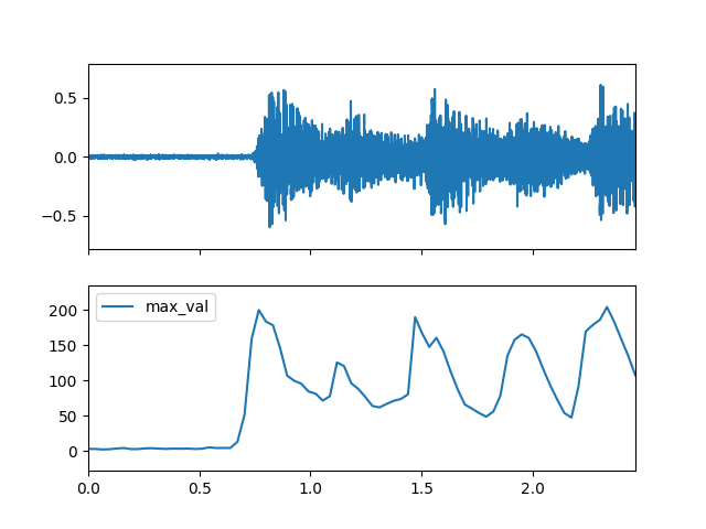
- max(m_data_arr)
Compute the spectral max feature.
- Parameters
- m_data_arr: np.ndarray [shape=(…, fre, time)]
Spectrogram data.
- Returns
- val_arr: np.ndarray [shape=(…, time)]
max value for each time
- fre_arr: np.ndarray [shape=(…, time)]
max frequency for each time
Examples
Read chord audio data
>>> import audioflux as af
>>> audio_path = af.utils.sample_path('guitar_chord1')
>>> audio_arr, sr = af.read(audio_path)
Create BFT-Linear object and extract spectrogram
>>> from audioflux.type import SpectralFilterBankScaleType, SpectralDataType
>>> import numpy as np
>>> bft_obj = af.BFT(num=2049, samplate=sr, radix2_exp=12, slide_length=1024,
>>>                data_type=SpectralDataType.MAG,
>>>                scale_type=SpectralFilterBankScaleType.LINEAR)
>>> spec_arr = bft_obj.bft(audio_arr)
>>> spec_arr = np.abs(spec_arr)
Create Spectral object and extract max feature
>>> spectral_obj = af.Spectral(num=bft_obj.num,
>>>                            fre_band_arr=bft_obj.get_fre_band_arr())
>>> n_time = spec_arr.shape[-1]  # Or use bft_obj.cal_time_length(audio_arr.shape[-1])
>>> spectral_obj.set_time_length(n_time)
>>> max_val_arr, max_fre_arr = spectral_obj.max(spec_arr)
Display plot
>>> import matplotlib.pyplot as plt
>>> from audioflux.display import fill_plot, fill_wave
>>> fig, ax = plt.subplots(nrows=2, sharex=True)
>>> fill_wave(audio_arr, samplate=sr, axes=ax[0])
>>> times = np.arange(0, len(max_val_arr)) * (bft_obj.slide_length / bft_obj.samplate)
>>> fill_plot(times, max_val_arr, axes=ax[1], label='max_val')
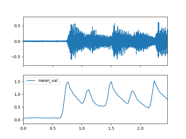
- mean(m_data_arr)
Compute the spectral mean feature.
- Parameters
- m_data_arr: np.ndarray [shape=(…, fre, time)]
Spectrogram data.
- Returns
- val_arr: np.ndarray [shape=(…, time)]
mean value for each time
- fre_arr: np.ndarray [shape=(…, time)]
mean frequency for each time
Examples
Read chord audio data
>>> import audioflux as af
>>> audio_path = af.utils.sample_path('guitar_chord1')
>>> audio_arr, sr = af.read(audio_path)
Create BFT-Linear object and extract spectrogram
>>> from audioflux.type import SpectralFilterBankScaleType, SpectralDataType
>>> import numpy as np
>>> bft_obj = af.BFT(num=2049, samplate=sr, radix2_exp=12, slide_length=1024,
>>>                data_type=SpectralDataType.MAG,
>>>                scale_type=SpectralFilterBankScaleType.LINEAR)
>>> spec_arr = bft_obj.bft(audio_arr)
>>> spec_arr = np.abs(spec_arr)
Create Spectral object and extract mean feature
>>> spectral_obj = af.Spectral(num=bft_obj.num,
>>>                            fre_band_arr=bft_obj.get_fre_band_arr())
>>> n_time = spec_arr.shape[-1]  # Or use bft_obj.cal_time_length(audio_arr.shape[-1])
>>> spectral_obj.set_time_length(n_time)
>>> mean_val_arr, mean_fre_arr = spectral_obj.mean(spec_arr)
Display plot
>>> import matplotlib.pyplot as plt
>>> from audioflux.display import fill_plot, fill_wave
>>> fig, ax = plt.subplots(nrows=2, sharex=True)
>>> fill_wave(audio_arr, samplate=sr, axes=ax[0])
>>> times = np.arange(0, len(mean_val_arr)) * (bft_obj.slide_length / bft_obj.samplate)
>>> fill_plot(times, mean_val_arr, axes=ax[1], label='mean_val')
- var(m_data_arr)
Compute the spectral var feature.
- Parameters
- m_data_arr: np.ndarray [shape=(…, fre, time)]
Spectrogram data.
- Returns
- val_arr: np.ndarray [shape=(…, time)]
var value for each time
- fre_arr: np.ndarray [shape=(…, time)]
var frequency for each time
Examples
Read chord audio data
>>> import audioflux as af
>>> audio_path = af.utils.sample_path('guitar_chord1')
>>> audio_arr, sr = af.read(audio_path)
Create BFT-Linear object and extract spectrogram
>>> from audioflux.type import SpectralFilterBankScaleType, SpectralDataType
>>> import numpy as np
>>> bft_obj = af.BFT(num=2049, samplate=sr, radix2_exp=12, slide_length=1024,
>>>                data_type=SpectralDataType.MAG,
>>>                scale_type=SpectralFilterBankScaleType.LINEAR)
>>> spec_arr = bft_obj.bft(audio_arr)
>>> spec_arr = np.abs(spec_arr)
Create Spectral object and extract var feature
>>> spectral_obj = af.Spectral(num=bft_obj.num,
>>>                            fre_band_arr=bft_obj.get_fre_band_arr())
>>> n_time = spec_arr.shape[-1]  # Or use bft_obj.cal_time_length(audio_arr.shape[-1])
>>> spectral_obj.set_time_length(n_time)
>>> var_val_arr, var_fre_arr = spectral_obj.var(spec_arr)
Display plot
>>> import matplotlib.pyplot as plt
>>> from audioflux.display import fill_plot, fill_wave
>>> fig, ax = plt.subplots(nrows=2, sharex=True)
>>> fill_wave(audio_arr, samplate=sr, axes=ax[0])
>>> times = np.arange(0, len(var_val_arr)) * (bft_obj.slide_length / bft_obj.samplate)
>>> fill_plot(times, var_val_arr, axes=ax[1], label='var_val')
