audioflux.cqcc
- audioflux.cqcc(X, cc_num=13, rectify_type=CepstralRectifyType.LOG, cqt_num=84, samplate=32000, low_fre=32.70319566257483, slide_length=None, bin_per_octave=12, window_type=WindowType.HANN, normal_type=SpectralFilterBankNormalType.AREA, is_scale=True)
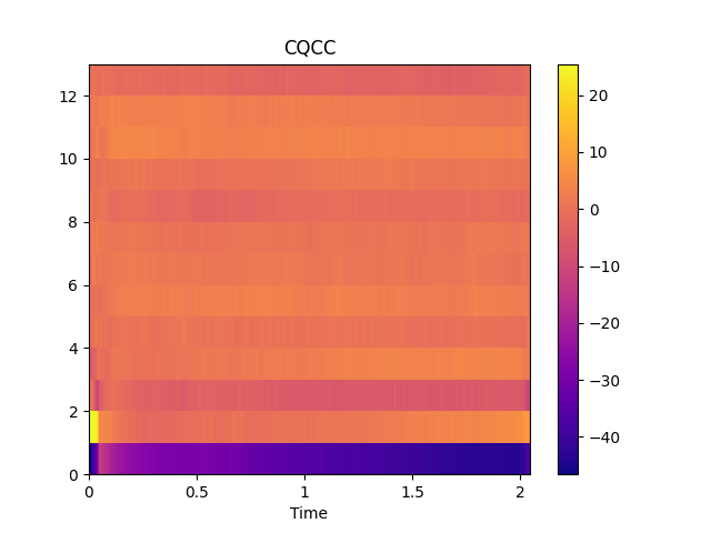
Constant-Q cepstral coefficients (CQCCs)
Note
We recommend using the CQT class, you can use it more flexibly and efficiently.
- Parameters
- X: np.ndarray [shape=(…, n)]
audio time series.
- cc_num: int
number of GTCC to return.
- rectify_type: CepstralRectifyType
cepstral rectify type
- cqt_num: int
Number of cqt frequency bins to generate, starting at low_fre.
- samplate: int
Sampling rate of the incoming audio.
- low_fre: float or None
Lowest frequency.
- slide_length: int or None
Window sliding length.
If slide_length is None, then
slide_length = fft_length / 4- bin_per_octave: int
Number of bins per octave.
- window_type: WindowType
Window type for each frame.
See:
type.WindowType- normal_type: SpectralFilterBankNormalType
Spectral filter normal type. It determines the type of normalization.
- is_scale: bool
Whether to use scale.
- Returns
- out: np.ndarray [shape=(…, cc_num, time)]
The matrix of CQCCs
- fre_band_arr: np:ndarray [shape=(fre,)]
The array of cqt frequency bands
Examples
Read 220Hz audio data
>>> import audioflux as af
>>> audio_path = af.utils.sample_path('220')
>>> audio_arr, sr = af.read(audio_path)
Extract cqcc data
>>> cc_arr, _ = af.cqcc(audio_arr, samplate=sr)
Show plot
>>> import matplotlib.pyplot as plt
>>> from audioflux.display import fill_spec
>>> import numpy as np
>>>
>>> # calculate x-coords
>>> audio_len = audio_arr.shape[-1]
>>> x_coords = np.linspace(0, audio_len/sr, cc_arr.shape[-1] + 1)
>>>
>>> fig, ax = plt.subplots()
>>> img = fill_spec(cc_arr, axes=ax,
>>>                 x_coords=x_coords, x_axis='time',
>>>                 title='CQCC')
>>> fig.colorbar(img, ax=ax)