audioflux.bfcc
- audioflux.bfcc(X, cc_num=13, rectify_type=CepstralRectifyType.LOG, bark_num=128, radix2_exp=12, samplate=32000, slide_length=None, low_fre=None, high_fre=None, window_type=WindowType.HANN)
Bark-frequency cepstral coefficients (BFCCs)
- Parameters
- X: np.ndarray [shape=(…, n)]
audio time series.
- cc_num: int
number of BFCC to return.
- rectify_type: CepstralRectifyType
cepstral rectify type
- bark_num: int
Number of bark frequency bins to generate, starting at low_fre.
- radix2_exp: int
fft_length=2**radix2_exp- samplate: int
Sampling rate of the incoming audio.
- slide_length: int or None
Window sliding length.
If slide_length is None, then
slide_length = fft_length / 4- low_fre: float or None
Lowest frequency.
- high_fre: float or None
Highest frequency. Default is 16000(samplate/2).
- window_type: WindowType
Window type for each frame.
See:
type.WindowType
- Returns
- out: np.ndarray [shape=(…, cc_num, time)]
The matrix of BFCCs
- fre_band_arr: np:ndarray [shape=(fre,)]
The array of Bark frequency bands
Examples
Read 220Hz audio data
>>> import audioflux as af
>>> audio_path = af.utils.sample_path('220')
>>> audio_arr, sr = af.read(audio_path)
Extract bfcc data
>>> cc_arr, _ = af.bfcc(audio_arr, samplate=sr)
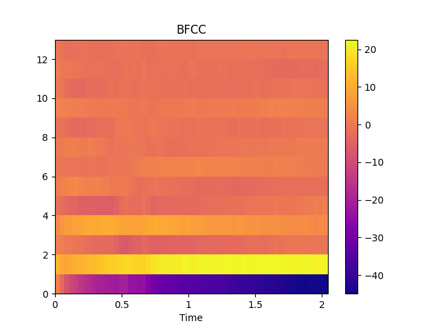
Show plot
>>> import matplotlib.pyplot as plt
>>> from audioflux.display import fill_spec
>>> import numpy as np
>>>
>>> # calculate x-coords
>>> audio_len = audio_arr.shape[-1]
>>> x_coords = np.linspace(0, audio_len/sr, cc_arr.shape[-1] + 1)
>>>
>>> fig, ax = plt.subplots()
>>> img = fill_spec(cc_arr, axes=ax,
>>>                 x_coords=x_coords, x_axis='time',
>>>                 title='BFCC')
>>> fig.colorbar(img, ax=ax)